Thesis and Viva
It’s been quite a year for me! I got a new job almost a year ago, wrote up my thesis, moved to a new city and I am about to move house again. Oh, and I just ...
Differential equations are central to the study of the natural world. They describe everything from the flow of fluids through pipes to the evolution of electrons in boxes. These equations naturally get very complicated very quickly thus we must put down our sharp pencils and turn to the more bluntened approach (albeit vastly more powerful) of numerical methods.
In this series I will explore how to solve Differential equations using computers and the fascinating methods which have been developed to solve the most complicated of these devils. We shall explore methods such as Parallel computing and Machine Learning , examine different approaches such as Density Matrix Renormalization Group and investigate how these approaches compare to one another.
We begin these posts with some simple ways to solve Ordinary Differential Equations (ODE’s). We could solve these problems analytically however whilst some ODE’s can be solved this way most cannot. Most differential equations that are useful to us are not solvable analytically, in fact we are not sure that a solution even exists at all points (Navier Stokes etc). However we are saved (as always) by the existence of computers. We can numerically solve these equations to find an approximate answer. The most basic version of this is the first order finite difference method or Euler method, using this method we can solve first order initial Value problems which take the form
\[ \frac{dy}{dt} = f(t,y) \quad \text{,} \quad y(t_0) = y_0.\] As we can evaluate both the derivative and the function on the LHS at the initial point we can use this information to determine an approximation to the derivative at a time step slightly into the future. The important question here is why can we do this. The answer is finite difference, an approximation to the derivative given by \[ \frac{dy}{dt} \approx \frac{y(t+h) - y(t)}{h}.\] We know this from Newtonian calculus, we also know that the smaller we make h the better the approximation becomes. This will help us when we come to code this up and look at different ODE's to solve. For now though the theory is that we can re arrange this into the solution we want \( y(t+h) \) and make it equal to the things we know (the rest of the equation helpfully) \[ y(t+h) \approx \frac{dy}{dt} + h y(t_0).\] This can now be iterated upon to give us the next point in the calculation, bringing us to the well known formula for Euler's method \[ y_{t+1} = f(t,y(t)) + h y(t).\] This is a great start but how good is it exactly. Well we can answer that question quite easily by coding this up in our language of choice. Currently I mainly work in python so that's what I will use here. The basic structure will be the same for most languages unless you want to use some weird language like Haskell (good luck though)The equation we would like to solve is
\[ \frac{dy}{dt} = y \quad \text{,} \quad y(0) = 1. \] A simple differential equation and so one which is easy to solve, the solution to which is \[ y(t) = e^t. \] Now we can turn to our algorithm defined above and see how well it performs. The code we need is simple but i will go through it nonetheless, firstly our importsfrom math import e # The exponential function for the solution
import numpy as np # Numpy for manipulation of arrays
import matplotlib.pyplot as plt # For plotting the result
Next we define all of the variables and constants we need and implement the inital conditions
h = 1.0 # large step size at first

Y = []
Y.append(1)

Y_true = []
Y_true.append(e**0) # Initial Condition
t_lst = []
t_lst.append(0)# Initial Condition
Now we implement the algorithm
for i in range(0,5):
	Y.append(Y[i] + h*Y[i]) # Forward Euler method
	t_lst.append((i+1)*h)
for i in range(50):
	#Using Smaller step size for the true solution to approximate the continuum
	Y_true.append(e**((i+1)*0.1))
	t_lstT.append((i+1)*0.1)
from math import sin, cos
import numpy as np
import matplotlib.pyplot as plt

h1 = 0.3

Y1 = [];U1 = [];t_lst1 = []


#Initial Conditions
Y1.append(1)
U1.append(1)
t_lst1.append(0)

for i in range(0,100):
	U1.append(U1[i] - Y1[i]*h1)
	Y1.append(Y1[i] + U1[i]*h1)
	t_lst1.append(h1*i)


plt.plot(t_lst1,Y1,label='h=0.3')
plt.xlim((0,20))
plt.ylim((-20,20))
plt.legend()
plt.xlabel("Time")
plt.ylabel("y(t)")
plt.title("Euler Method for Second Order ODE's")
plt.show()
Which produces the result
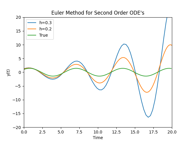
As can be easily seen the Euler method breaks down for this oscillating solution but why is this? Can we predict if this is going to occur? Are there any improvements we can make to stop this from happening or at least reduce the error.
All of these and more will be answered in my next posts.
![]()
It’s been quite a year for me! I got a new job almost a year ago, wrote up my thesis, moved to a new city and I am about to move house again. Oh, and I just ...
First Quantum Computing Hackathon
A Bog Standard Introdution to Quantum Computing As with most introductions to scientific books and blogs there always has to be sections that are repeated ev...
Now that we have dealt with the ordinary differential equations we can go one of two ways. We can explore how to solve all types of these ODE’s and keep on s...
Quantum Computing is posed to become one of the most useful technologies invented. It boasts algorithms that can outperform some of the best classical algori...
Previously we discussed how to solve some simple ODE’s and looked at coding a simple forward Euler algorithm. However we found that the solution we used does...
Differential equations are central to the study of the natural world. They describe everything from the flow of fluids through pipes to the evolution of elec...