Thesis and Viva
It’s been quite a year for me! I got a new job almost a year ago, wrote up my thesis, moved to a new city and I am about to move house again. Oh, and I just ...
Previously we discussed how to solve some simple ODE’s and looked at coding a simple forward Euler algorithm. However we found that the solution we used doesn’t always work. This will be a feature of these posts, finding where our current methods fail and looking for ways to improve them.
To understand why the Euler method failed we must first understand where it comes from. I mentioned in the previous post that it comes from a discretization, which is a simple enough explanation but it hides quite a lot. When we discretise a system we naturally are throwing away some of the information in that system. There is a vast literature on this so I will only be brief in my explanation and point the interested reader towards some more extensive reviews of the topic. Discretization comes from the Taylor expansion of the function itself. \[ f(x) = \frac{f(0)}{0!} + \frac{f'(0) x}{1!} + \frac{f'' (0) x^2}{2!} + ...\] If we truncate this to second order in \(x\) then we find the definition of the derivative from the previous post. However there are many more terms in this series to take account of. This is the main problem, when these terms become large then we can no longer discount them. If we do (as we did in the Euler method) we are punished and the solution our method produces can be vastly different from the true solution, see previous post. To account for this the most obvious thing to do is to include more terms. These types of methods are called higher order methods and are one of the ways we can improve the accuracy of our solutions. The inclusion of higher order terms from the Taylor expansion leads to a family of methods known as the Runge-Kutta methods. These include one of the most used methods for solving ODE's the 4th order Runge-Kutta (or RK4 for short). There are lots of other methods for solving ODE's but i do not want to dwell on them too much so I shall leave a link to some of them for anyone who wants to look into them more. Here I shall look at the derivation of the second and fourth order Runge-Kutta method and compare the two. We consider the first-order ODE system, \[ \frac{dy}{dt} = f(t,y(t)). \] Since we want a second order method we should start with the Taylor expansion of a function \[ y(t+h) = y(t) + h y'(t) + \frac{h^2}{2} y'' (t) + O (h^3).\] We can replace the first order derivative with the RHS of our ODE system, we can also replace the second order derivative with a chain rule expansion \[ \frac{d^2y}{dt^2} = \frac{df}{dt} + \frac{df}{dy} \frac{dy}{dt}.\] The Taylor expansion becomes \[ y(t+h) = y(t) + h f(t,y) + \frac{h^2}{2} [\frac{df}{dt} + \frac{df}{dy} \frac{dy}{dt}], \] \[ y(t+h) = y(t) + \frac{h}{2} f(t,y) + \frac{h}{2} [f(t,y) + h \frac{df}{dt} + h \frac{df}{dy} \frac{dy}{dt}],\] We now recall the taylor expansion for a multi varied function \[ f(t+h, y+k) = f(t,y) + h \frac{\partial f}{\partial t} + k \frac{\partial f}{\partial y} + ... \] Thus we can interpret the term in brackets as a multivaried taylor expansion, thus getting the following \[ y(t+h) = y(t) + \frac{h}{2} f(t,y) + \frac{h}{2} f(t+h,y+h f(t,y)) + O(h^3).\] Translating this quickly into a numerical method we have \[ y_{n+1} = y_n + \frac{h}{2}(k_1 + k_2), \] where, \[ k_1 = f(t_n,y_n) \quad \text{and} \quad k_2 = f(t_n + h , y_n + h k_1 ).\] This is the classical second-order Runge-Kutta method. It is also known as Heun’s method or the improved Euler method. We can compare this to the Euler method to see how much better this is.We must say here that there is a whole family of solutions to the above equations. These are all valid Runge-Kutta methods which are all equivalent to one another. So if you see an RK2 or RK4 algorithm that looks slightly different remember it is just one of a family of the RK2/4 algorithms.
###### Initialize the parameters and arrays ######

Y2 = [];U2 = [];T2  = []

# Initial conditions

Y2.append(0);U2.append(1/pi);T2.append(0)

h2 = 0.1

for i in range(0,500):
  U2.append(U2[i] - 0.5*h2*(2*Y2[i] + h2*Y2[i]))
  Y2.append(Y2[i] + 0.5*h2*(2*U2[i] + h2*U2[i]))

  T2.append(h2*i)
As we can see the set up of this code is very similar to the Euler method just now with a few more steps in the calculation of the next time step. Comparing this to the Euler method we developed in the last Post
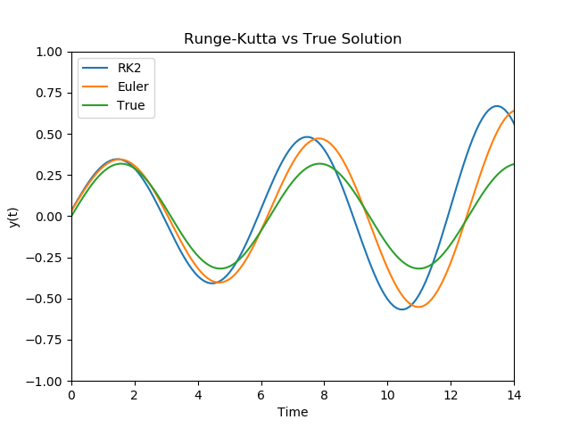
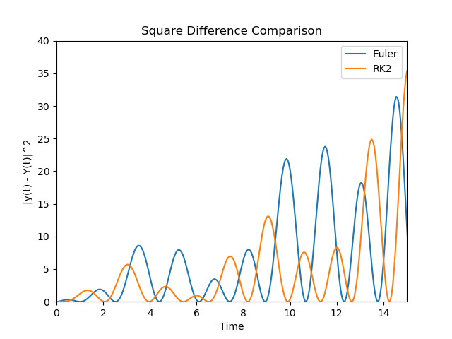
As we can see the Runge-Kutta methods here are much closer to the true Solution than the Euler method. In terms of difference we can plot the squared difference from the truse solution
#Initialize arrays
Y4 = [];U4 = [];T4  = []
Y4.append(0);U4.append(1/pi);T4.append(0)
#RK4 Loop
for i in range(0,200):

    k1_Y = h4*U4[i]
    k1_U = -1*h4*Y4[i]

    k2_Y = h4*(U4[i] + 0.5 * k1_U)
    k2_U = -1*h4*(Y4[i] + (0.5 * k1_Y))

    k3_Y = h4*(U4[i] + 0.5 * k2_U)
    k3_U = -1*h4*(Y4[i] + (0.5 * k2_Y))

    k4_Y = h4*(U4[i] + k3_U)
    k4_U = -1*h4*(Y4[i] + k3_Y)

    Y4.append(Y4[i] + (1/6) * (k1_Y + 2*k2_Y + 2*k3_Y + k4_Y))
    U4.append(U4[i] + (1/6) * (k1_U + 2*k2_U + 2*k3_U + k4_U))
    T4.append(h4*i)
Now we can compare the results from our RK4 algorithm to the true solution
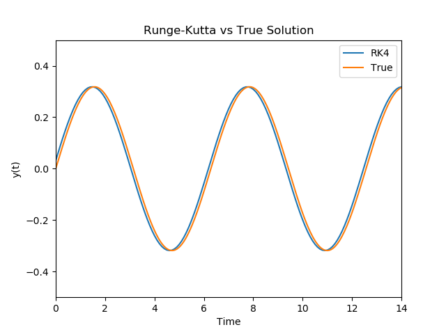
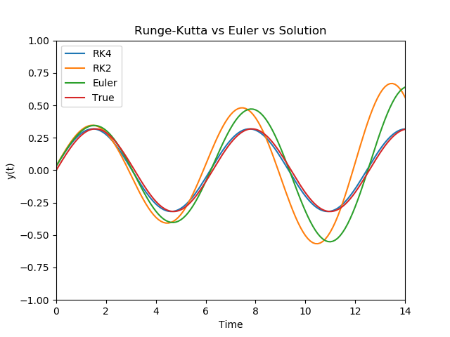
As we see above the RK4 method is very close to the True solutions and when we compare it to the other methods we have discussed here
Now that we have looked at some higher order methods we shall turn to a subject not quite as exciting but non the less important. We shall examine Error analysis and stability of these algorithms as it will be important to consider these concepts when we look at algorithms in the future.
![]()
It’s been quite a year for me! I got a new job almost a year ago, wrote up my thesis, moved to a new city and I am about to move house again. Oh, and I just ...
First Quantum Computing Hackathon
A Bog Standard Introdution to Quantum Computing As with most introductions to scientific books and blogs there always has to be sections that are repeated ev...
Now that we have dealt with the ordinary differential equations we can go one of two ways. We can explore how to solve all types of these ODE’s and keep on s...
Quantum Computing is posed to become one of the most useful technologies invented. It boasts algorithms that can outperform some of the best classical algori...
Previously we discussed how to solve some simple ODE’s and looked at coding a simple forward Euler algorithm. However we found that the solution we used does...
Differential equations are central to the study of the natural world. They describe everything from the flow of fluids through pipes to the evolution of elec...