Numerical Methods 3 - Introduction to Partial Differential Equations

Now that we have dealt with the ordinary differential equations we can go one of two ways. We can explore how to solve all types of these ODE’s and keep on solving them until the cows come home……. or we can move onto something a little different. We can extend our understanding of Differential Equations by exploring systems that involve more than one variable and derivative thereof. This path will lead us to much MUCH more interesting things such as Quantum Physics and Fluid Simulation.

We must now begin with a short but needed discussion on what exactly Partial Differential Equations (PDE's) are, this isn't exactly a new thing and something that has been done thousands of times (I shall leave links to other , possibly better, introductions) but for completeness I believe I should put this here. To begin with I shall introduce what is known as the partial derivative (again this can be a huge topic but link link link blah blah blah). When the functions we want to deal with are functions of more than one variable we can take derivatives wrt each of the different variables independently of one another. We do this by keeping the other variables constant and varying the one we are interested in. This is called taking a partial derivative. Partial differentials naturally lead to the idea of partial differential equations, differential equations are the natural extensions of ordinary differential equations to functions of multiple variables. These equations can be solved analytically however much like ODE’s the equations or families of equations that can be solved are usually the exception rather than the rule . The amount of PDEs is also much larger than ODE’s. Hence we need to turn towards numerical methods to solve these equations. PDEs are the most common differential equations which is solved in science and engineering and this class of equations covers most of the important equations in science ( Schroedinger equation, Napier stokes , Burgers equation etc.) hence a lot of work is put into improving the numerical methods for solving these equations.

Where and why are they used

PDEs are almost all pervasive in science, engineering and beyond. They appear in everything from fundamental physics (Maxwell's Equations) to modeling traffic flow (Burgers Equation). This wide range of applications can be put down to the general nature of differential equations. In most of our world we can describe things by how they change much easier than how they actually are. We may not know why the traffic jam occurred exactly but we can certainly tell the changes that occurred because of it.

How to Solve them

Analytical solutions to PDEs are few and far between to be honest. We can certainly spend a long time (I did in my degree) discussing exactly how to solve these equations analytically using various methods (separation of variables etc ) and find general solutions. However there are many PDE's (most of the ones which describe real life in fact) which do no have what we call closed solutions. These are solutions which can be written down exactly on a (somewhat large in some cases) piece of paper. So, we would need a different approach to solve these problems. As before we turn to our trusty computer and ask it very nicely to solve it for us. This is where it may get a little complicated. Since there are now more variables to deal with the complexity of the solver will be much higher. As a general rule PDEs are much trickier to solve than ODE's and often need much more complicated solvers to achieve a sufficiently high degree of accuracy.

Note

I have written up an example of how to solve a PDE analytically. As it can be seen there is quite a lot of work to solve a simple equation. I shall be going through those more complicated algorithms over the next couple of posts however here I would like to give an example of how to solve a simple PDE with pen and paper and an example of where you cannot solve a PDE and must use a computer to solve it. The first two methods I shall explore are both similar and will be easy for someone who has only explored the ODE solvers to understand.

Finite Difference Method

The finite difference method is the simplest algorithm for solving PDEs that anyone could come up with as with ODE's we examined before we discretize everything we can. A Prime example of this discretization is to solve the Laplace Equation which describes a steady state heat equation since the RHS of this equation is 0. \[ \frac{\partial^2 T}{\partial x^2} + \frac{\partial^2 T}{\partial y^2} = 0\] Replacing the differential with their finite difference approximation giving us \[ T_{i+1,j} + T_{i-1,j} + T_{i,j+1} + T_{i,j-1} - 4 T_{i,j} = 0\] Note that here I have set the lattice space of x and y equally so they exactly cancel out making the equations easier to deal with. Now that we have an expression for the discrete version of the PDE we can turn this into a Linear Algebra problem which can be solved using methods readily available in programs such as MATLAB and Scipy. The form of the problem we are aiming for is \( Ax = B\) where \( A\) is a Matrix and \(B\) is a column vector which contains the Initial conditions. We now wish to solve this for \(x\) so first we must recast the discretized PDE into a Matrix and the Initial conditions into a column vector T. This can be achieved by taking the matrix of initial conditions that is \[ \begin{bmatrix} T_{0,0} & T_{0,1} & ... & T_{0,N} \\ T_{1,0} & T_{1,1} & ... & T_{1,N} \\ ... & ... & ... & ... \\ T_{N,0} & T_{N,1} & ... & T_{N,N} \end{bmatrix} \] we now put this matrix into a row major order to create the initial state vector \[ \begin{bmatrix} T_{0,0}\\ T_{0,1}\\ T_{0,2}\\ ... \\ ... \\ T_{1,0}\\ ...\\ T_{N,N} \end{bmatrix} \] With this vector in mind we can construct a matrix that multiplies a general vector \(X\) which is of the same form as \(T\). This matrix equation is now equivalent to the discretized version of the PDE but now describes the area which we are concerned with. This matrix takes the form \[ \begin{bmatrix} 4 & -1 & 0 & -1 & 0 & 0 & ... \\ -1 & 4 & -1 & 0 & -1 & 0 & ... \\ 0 & -1 & 4 & 0 & 0 & -1 & ... \\ -1 & 0 & 0 & 4 & -1 & 0 & ... \\ 0 & -1 & 0 & -1 & 4 & -1 & ... \\ 0 & 0 & -1 & 0 & -1 & 4 & ... \\ ... & ... & ... & ... & ... & ... & ... \end{bmatrix} \]

Now that we have the matrix equation we can code this up relatively easily. MATLAB is a perfect language to solve this problem as it is built to handle matrices easily and has very accurate inbuilt Linear Algebra solvers we make use of these solvers to code up this algorithm. To create the Matrix that defines the discrete PDE we have the following.

% A Script to solve the Laplace Equation using a Finite Difference Method

% First need to define the laplacian matrix. We will be turning this into
% a linear algebra problem of solving for x in Ax = B

clear;clc;

N = 60; % Number of points in the grid

L_center = eye(N).*4;

for I = 1:N-1
    L_center(i,i+1) = -1;
    L_center(i+1,i) = -1;
end

L_offdiag = eye(N) .* -1;  

L_Other = zeros(N);
A = zeros(N,N,N,N);
for I = 1:N-1
    A(i,i,:,:)      = L_center;
    A(i,i+1,:,:)    = L_offdiag;
    A(i+1,i,:,:)    = L_offdiag;
end

% reshape:
S = size(A);
L = reshape(permute(A,[1,4,2,3]),N*S(1:2));

Once that is setup we can construct the Initial condition (and Boundary condition) vector

% Now we have the the discretized version of the laplacian we can create
% the vector which describes the initial state of the system.

T = zeros(N*N,1);

for I = 1:N-1
    T(i,1) = 100;
    T((N-1)*N + i,1) = 100;
end

These initial conditions set the left and right sides of a square to 100 degrees and the other sides to 0. Now we can solve the system we have created using linsolve and plot a 2d colourmap of the result.

tic;
X = linsolve(L,T);
toc;
% now reshape the vector and plot the result

Z = reshape(X,N,N);

[x,y] = meshgrid(1:N, 1:N);

surface(x,y,Z,'EdgeColor', 'black');
colorbar;

These calculations produce

In this simulation the grid was 60x60, we can investigate the scaling of this method by varying this producing the following results.

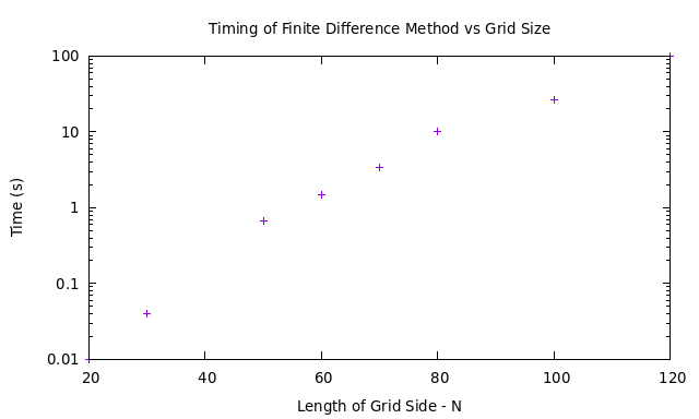
The logscale on the Y axis shows that this is an exponential scaling, meaning that if we want very accurate results even for this simple system our code will take quite some time to run.

Method of Lines

Another Method to solve PDEs is the Method of lines. This method still follows the thinking of discretization however this method relies on discretising only one of the coordinates and leaving the other one in the continuum. This leaves us with an ODE system to solve which is much easier to solve that the PDE that we had before. We know we can solve systems of ODE’s with highly accurate solvers such as RK4 (see previous posts) so these are the solvers that are used here.

To show how this works I shall, as always , show an example. For this example I shall use the diffusion or heat equation

[[ \frac{\partial u}{\partial t} = D \frac{\partial^2 u}{\partial x^2}\]]

Discretising the RHS of the equation using the usual finite difference formula, we now have

\[ \frac{d u_i}{dt} = D \frac{u_{i+1} - 2 u_i + u_{i-1}}{\Delta x^2}\]

Now we have a system of ODEs which we know can be solved using Runge-Kutta Methods from the previous posts. Instead of using python we shall again use MATLAB to show another language but more importantly it has very accurate inbuilt solvers which can handle matrices very well. This helps us immensely since we can formulate the equations above in terms of matrices/vectors again.

Solving this problem in MATLAB we first have to define the problem in a different script.

function du = diff_eqs(t,u)

% parameters
global dx
D = 1;
dx2 = dx^2;
  xl=0.0;
  xu=1.0;
%
% PDE
  n=length(u);
  dx2=((xu-xl)/(n-1))^2;
 for j = 1:n
    if(j==1)        du(j)=2.0*(u(j+1)-u(j))/dx2;
    elseif(j==n)    du(j)=2.0*(u(j-1)-u(j))/dx2;
    else            du(j) =  D * ((u(j+1) - 2.0*u(j) + u(j-1))/dx2);
    end
 end
 
 du = du';
 

end

In this file we have defined the differential in the bulk and at the edges. The system will incur some errors at the edges since (as can be seen above) the difference equation is not complete. Now that we have defined the equation to solve we can turn to putting this into MATLABs inbuilt solvers. I use ode45 the workhorse of MATLAB’s ODE library, to solve this equation. This function will use RK4 algorithm like we developed in the last post but with some optimization routines built in such as adaptive step etc.

% A Method of lines algorithm to solve differential equations

% Initial Conditions
clear;clc;
N = 41;

for j=1:N
    U0(j) = sin((pi/1.0)*(j-1)/(N-1)); % Initial condition
end

%timing
ti = 0.0;
tf = 1.0;
tout=linspace(ti,tf,N);

% ODE integration
 
reltol=1.0e-05; abstol=1.0e-05;
options=odeset('RelTol',reltol,'AbsTol',abstol);

[t,u]=ode15s(@diff_eqs,tout,U0,options); %Perform the integration

The result of this code is thus

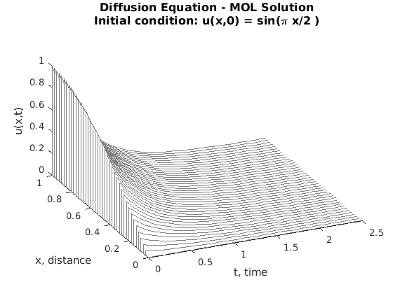
From this graph we can see ( as you have probably guessed by now) that the Method of Lines is very accurate in time but much less accurate in its discretization of space.

In this last post we have explored some of the more basic algorithms for solving differential equations. However these are only really useful for solving scientific problems, they do not generalise well to higher dimensions and different geometries. Whilst the Finite difference method is fine for square or rectangular lattices different more complex geometries will be problematic to implement with this method. Accuracy at the edges will have to be sacrificed if approximations such as interpolation will need to be made. The Method of lines is also tricky to put onto a complex geometry since it uses basic ODE solvers. It is also only accurate to the first order in the discretized variables meaning that the entire algorithm is this order in error since this is the largest error.

There are many other algorithms that we could discuss for solving scientific ODE’s which often concern simple geometries and limited dimensions. There are more complex algorithms which can be implemented such as the split step Fourier method. I will discuss these in an interim post that will come later. For now I shall move on with discussing algorithms which can handle more complex geometries. These methods will be the Finite Element Method and the Finite Volume Method.

2023

Thesis and Viva

It’s been quite a year for me! I got a new job almost a year ago, wrote up my thesis, moved to a new city and I am about to move house again. Oh, and I just ...

2022

Quantum Computing Hackathon 2022

First Quantum Computing Hackathon

2020

Numerical Methods 1 - Introduction and Euler Method

Differential equations are central to the study of the natural world. They describe everything from the flow of fluids through pipes to the evolution of elec...